probability-distributions-and-random-variables

Fri Jul 03 2026

Why Numbers Beat Sets

Up to Chapter 2 an event is a set of outcomes, and the only tools are set operations: union, intersection, complement. That is limiting. You can intersect "it rains" with "I carry an umbrella", but you cannot add two events, or XOR them, or double one. There is no arithmetic on sets of outcomes.

A random variable fixes this by mapping each outcome to a number:

$X : \Omega \to \mathbb{R}.$

Now the outcomes are numbers, so $X + Y$, $2X$, and $X \oplus Y$ all mean something, and each is itself a new random variable. That is the real reason random variables exist: they let you build new quantities out of old ones.

A random variable adds no randomness of its own. The randomness lives in the underlying experiment, the sample space $\Omega$. The variable relabels those outcomes as numbers, and in doing so it induces a new distribution on the numbers. Same randomness, new bookkeeping.

The simplest kind is an indicator random variable, which is 1 when some event happens and 0 otherwise. It answers a yes/no question as a number, and adding up indicators is how you count events.

The PMF: a Random Variable's Fingerprint

A discrete random variable, one whose range is finite or countable, is fully described by its probability mass function:

$p_X(x) = P(X = x).$

Read $P(X = x)$ as the probability of the event $\{\omega : X(\omega) = x\}$, all the outcomes the variable sends to $x$. The PMF lists, for each value the variable can take, how much probability lands there.

Two conditions make a function a valid PMF. It is nonnegative, $p_X(x) \ge 0$ for every $x$, since probabilities cannot go below zero. And it sums to 1 over the support, $\sum_x p_X(x) = 1$, since the variable takes some value with certainty.

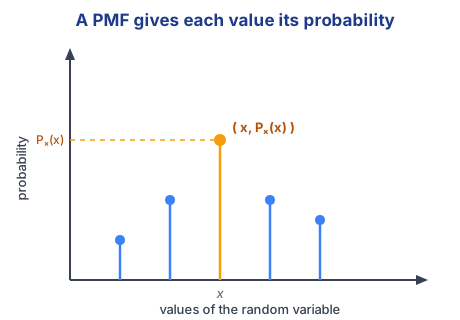
The PMF is what people mean by "the distribution of a discrete random variable". Hand me the PMF and I know everything probabilistic about $X$.

The Named Distributions

Four distributions do most of the work in this chapter. Two are worth knowing cold.

Bernoulli: one trial

$X \sim \text{Bern}(p)$ is a single trial with two outcomes, success and failure. It is the indicator of success:

$P(X = 1) = p, \qquad P(X = 0) = 1 - p.$

The failure probability $1 - p$ turns up so often it gets its own letter, $q = 1 - p$. That is the whole distribution. Every yes/no experiment with success chance $p$ is a Bernoulli.

Binomial: n independent trials

$X \sim \text{Bin}(n, p)$ counts the successes in $n$ independent Bernoulli$(p)$ trials, all sharing the same $p$:

$P(X = k) = \binom{n}{k} p^{k} (1-p)^{n-k}.$

The story reads straight off the formula. The factor $p^{k} q^{n-k}$ is the chance of one particular sequence with $k$ successes, and $\binom{n}{k}$ counts how many such sequences there are.

When $p = \tfrac{1}{2}$ the $p^{k} q^{n-k}$ factor is the same $1/2^{n}$ for every $k$, so the shape is carried entirely by $\binom{n}{k}$. That makes $\text{Bin}(n, \tfrac{1}{2})$ symmetric, peaking in the middle and tapering to the edges.

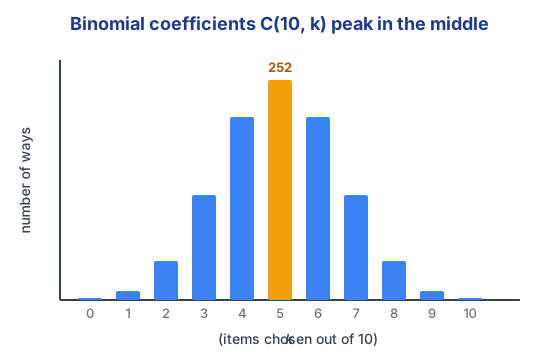
That peak is the same shape as a random walk's position and a two-dice sum, and why it peaks is worth its own note: random-walk-is-binomial.

Discrete Uniform and Hypergeometric, in brief

$X \sim \text{DUnif}(C)$ spreads probability evenly over a finite set $C$, so $P(X = x) = 1/|C|$ for each $x \in C$. It is the "no reason to prefer any value" baseline.

$X \sim \text{HGeom}(w, b, n)$ is the number of white items in a sample of $n$ drawn without replacement from a jar of $w$ white and $b$ black. You pull $n$ items in total, a mix of both colours, and $X = k$ counts how many of them are white:

$P(X = k) = \frac{\binom{w}{k}\binom{b}{n-k}}{\binom{w+b}{n}}.$

The numerator reads straight off that story: pick which $k$ of the $w$ white items landed in the sample, $\binom{w}{k}$, and which $n-k$ of the $b$ black ones filled the rest, $\binom{b}{n-k}$, over all $\binom{w+b}{n}$ ways to draw the sample.

The one thing to hold onto is the contrast with Binomial. Binomial is sampling with replacement, so the draws are independent and $p$ never moves. Hypergeometric is sampling without replacement, so each draw changes the composition of the jar and the draws are dependent. Reach for Binomial when the pool is effectively infinite, Hypergeometric when it is a fixed finite pool. Mixing them up is an easy slip: a "count the successes" problem is only Binomial if the trials are actually independent.

A clean way to picture the Hypergeometric is that every item carries two tags, its type (white or black) and its status (sampled or not). The count $k$ sits in the white-and-sampled cell.

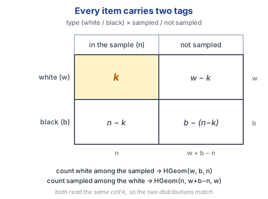
Swapping which tag you call "type" and which you call "sample" gives a distribution that reads differently but comes out equal. Why that symmetry holds is one I have parked in probability-open-questions.

The CDF: One Descriptor for Everything

The cumulative distribution function accumulates the PMF from the left:

$F_X(x) = P(X \le x).$

Its value at $x$ is the total probability at or below $x$. The CDF is the universal descriptor because it is defined for every random variable, discrete or continuous, while the PMF only makes sense for discrete ones. It always climbs from 0 to 1 and never decreases.

For a discrete variable the two hold the same information. The CDF is the running sum of the PMF, and the PMF is recovered as the size of each jump in the CDF, the jump at $x$ being exactly $p_X(x)$.

Building New Random Variables

Because a random variable is a function on $\Omega$, any function of it, $g(X)$, is again a function on $\Omega$, so it is another random variable. $X^{2}$, $2X$, and $|X|$ are all random variables in their own right.

This gives a handy technique for a variable whose distribution you do not recognize: express it as a one-to-one function of a variable you do know. A one-to-one $g$ relabels the values without merging any of them, so each new value inherits the probability of the old one it came from. That is the trick behind the random walk, whose position is a one-to-one relabelling of a Binomial count, worked in random-walk-is-binomial.

Two Category Errors to Avoid

Blitzstein calls these "sympathetic magic": treating a random variable as if it were its distribution, or as if it were a plain number.

The second slip is doubling. To get the PMF of $2X$ you cannot double the PMF of $X$. The values double, the probabilities do not. $P(2X = 4)$ equals $P(X = 2)$, since the probability stays with its outcome and only the label moves. Doubling the probabilities instead would not even leave them summing to 1.

What's Still Shaky

Three threads from this chapter I have not closed, parked in probability-open-questions: the Hypergeometric tag symmetry above, why the binomial coefficients across a row sum to $2^{n}$, and whether $X = Y$ as random variables forces them to map the underlying experiment identically. The deep dive on the peaked-distribution family lives in random-walk-is-binomial.