strauss-calibration-mental-model

Tue Mar 31 2026

In ecmult_multi, we model each algorithm's per-point cost as a linear function:

$\text{optime per point} = C + \frac{D}{n}$

where $C$ is the per-point floor and $D$ is the fixed overhead amortized over the batch. We compute $C$ and $D$ by fitting a linear regression to benchmark data in the $(1/n, \text{optime per point})$ coordinate system.

For Strauss, the calibration currently uses batches from $[2, 500]$, giving $C = 109$. But Strauss is only competitive up to about $n = 92$ — after that, it flatlines and starts degrading. If we calibrate on just $[2, 90]$ where Strauss is genuinely linear, we get $C = 104$.

So including the flatline region inflates C from 104 to 109. Why does including flat/degrading data push the intercept up?

The two coordinate systems

We measure Strauss performance in two different coordinate systems.

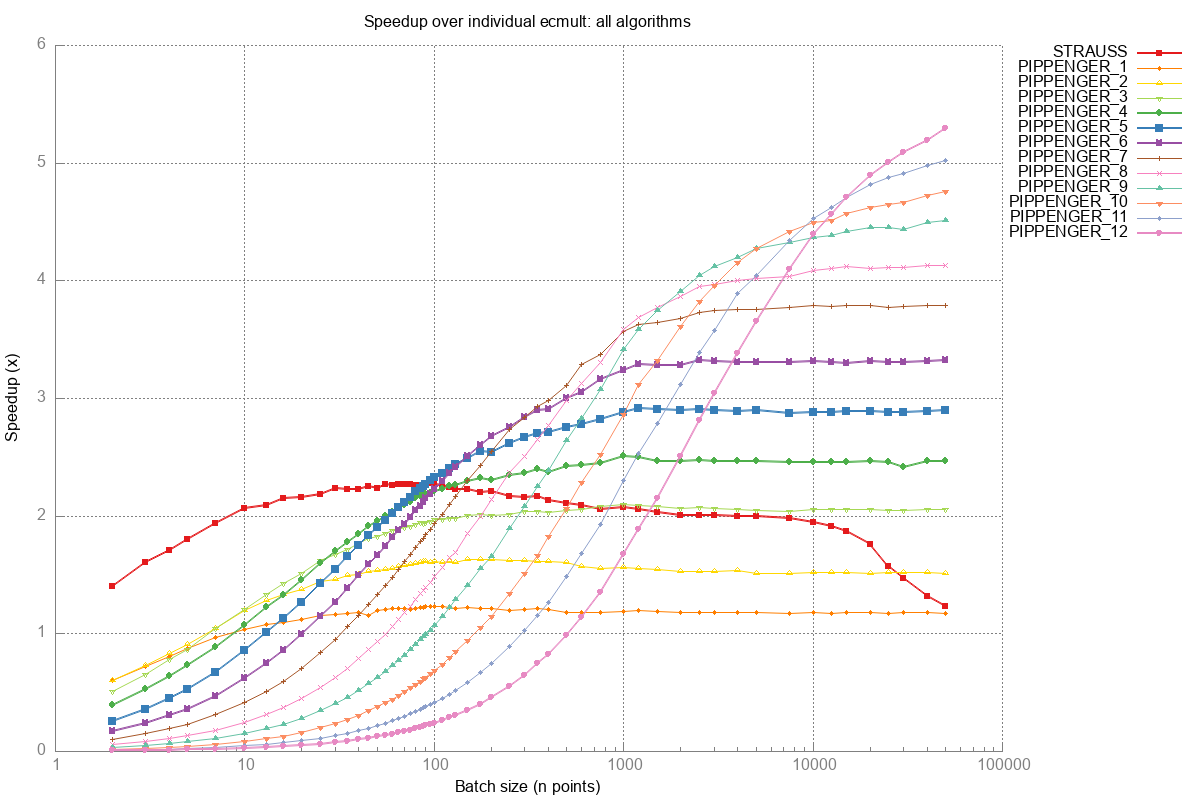
The speedup graph plots $(n, \text{speedup})$, where speedup $= \text{individual time} / \text{optime}$. So the y-axis is proportional to $1/\text{optime}$.

The regression space plots $(1/n, \text{optime per point})$, which is where the linear model $C + D/n$ lives. The y-axis here is just optime directly.

These two systems are related. Speedup is proportional to $1/\text{optime}$, so we're going from a $(1/\text{optime},\ n)$ system to an $(\text{optime},\ 1/n)$ system. Both axes invert. This means we can translate the shape of the speedup graph into the regression space — as long as we remember to flip both axes.

Note: we're measuring optime per point, not total optime. Total optime grows with $n$, so it wouldn't translate as cleanly. But per-point optime can flatline or decrease, and that's what makes this translation work.

Translating the Strauss curve

In the speedup graph, Strauss has two clear regions:

1. Increases from $n = 2$ to $n \approx 92$ — the algorithm gets faster per point as it amortizes its fixed overhead.
2. Flatlines from $n \approx 92$ to $n = 500$ — speedup stops improving. In reality it slightly decreases (Strauss degrades at large $n$), but it's close enough to flat for our reasoning.

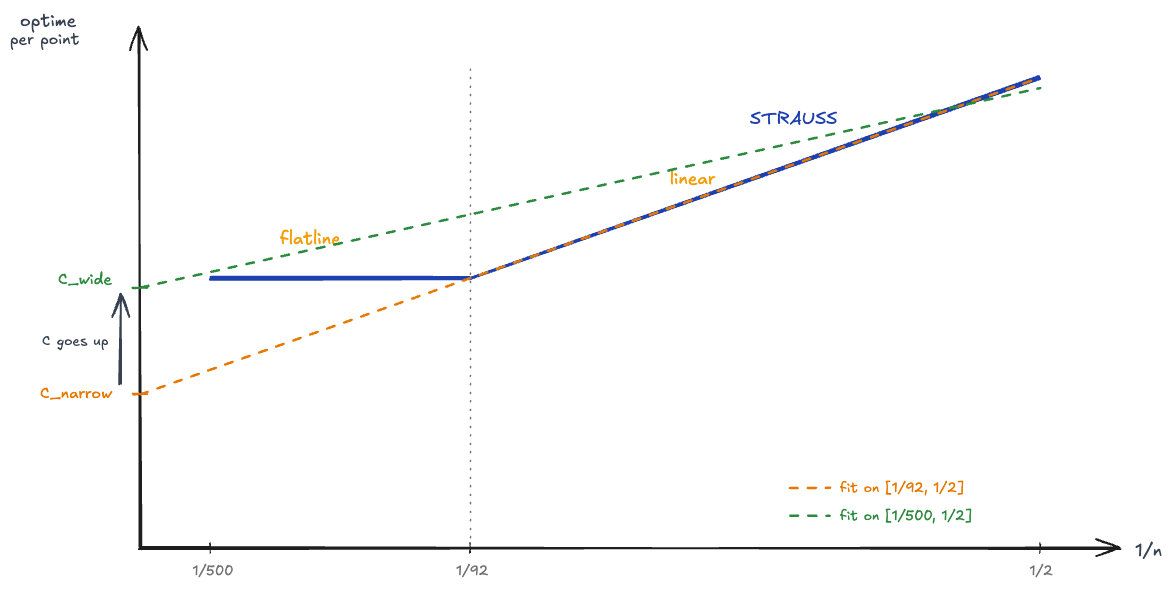
Now translate to the regression space $(1/n, \text{optime per point})$. The x-axis flips ($n \to 1/n$, so left-right reverses) and the y-axis inverts ($1/\text{optime} \to \text{optime}$, so up-down reverses). The translated curve has:

1. Flatline in $[1/500,\ 1/92]$ — this is now the left portion of the plot.
2. Increases in $[1/92,\ 1/2]$ — this is the right portion, rising steeply.

The increasing part was measuring $1/\text{optime}$ going up; flipping the y-axis means optime goes down in that region, so the rise becomes a decrease. And flipping the x-axis places it on the right. The flatline stays flat — roughly constant speedup means roughly constant optime.

Why the flatline pushes C up

Here's the key geometric picture.

When we fit a line on just the rising portion $[1/92, 1/2]$, we get a steep line. Extrapolating this line leftward toward $1/n = 0$ (the y-axis), the intercept $C_\text{narrow}$ ends up below the flatline level. This makes sense — the steep line is going down as it moves left, and it overshoots past where the data actually sits.

When we include the flatline points on the left side, the regression has to accommodate them. These points sit above the extrapolated line from the rising region. To fit them, the regression lifts its left end up (intercept $C$ increases) and becomes less steep (slope $D$ decreases).

In numbers:

• Narrow fit $[2, 90]$: $C_\text{raw} = 4.348$ us, scaled to $C = 104$
• Wide fit $[2, 500]$: $C_\text{raw} = 4.436$ us, scaled to $C = 109$

Including the flatline data pulls C up because the flatline sits above the linear extrapolation from the competitive region — Strauss never actually reaches the theoretical floor that the linear region predicts.

Why this inflation is useful

This C inflation turns out to be helpful. The algorithm selector picks the method minimizing $C + D/n$ using integer division. With $C = 109$ (inflated), the Strauss-to-Pippenger w5 crossover falls at exactly $n = 92$ in the C code — matching the empirical data almost perfectly. With $C = 104$ (accurate linear fit), the crossover moves to $n = 110$, causing ecmult_multi to keep picking Strauss well past where Pippenger w5 is faster.

Better statistical fit, worse real-world algorithm selection. The "bad" linear fit is actually a feature.