discrete-joint-distributions

Thu Jul 16 2026

Two marginals do not fix the joint

Suppose $X$ and $Y$ are each $\text{Bern}(1/2)$, and that is everything you know. What is $P(X=1, Y=1)$?

The natural first answer is 1/4:

The chain rule step is fine. The trap is the marked step, which replaced $P(Y=1 \mid X=1)$ with $P(Y=1)$. That replacement needs independence, and independence was never given. A counterexample: flip one fair coin, let $X=1$ for heads and $Y=1$ for tails. Both marginals are $\text{Bern}(1/2)$, yet $P(X=1, Y=1) = \tfrac12 \cdot 0 = 0$.

So the honest answer is "cannot be determined." Keep both marginals pinned at $\text{Bern}(1/2)$ and change only the relationship: the joint value is 0 when $Y = 1-X$ (one coin, opposite faces), 1/4 when independent (two separate coins), and 1/2 when $Y = X$ (one coin, same face). Same marginals, three different joints. Why this must happen, and the one-sample-space picture underneath it, is its own note: joint-distribution-mental-model.

The joint PMF as a 2D table

A joint probability mass function (PMF) can be visualized as a table: rows for $X$'s values, columns for $Y$'s, each cell holding $P(X=x, Y=y)$. The comma means "and", so every cell is an intersection event. There is no joint notation for "or": a union goes through inclusion-exclusion, $P(X{=}1 \text{ or } Y{=}1) = P(X{=}1) + P(Y{=}1) - P(X{=}1, Y{=}1)$, and even that needs a joint term.

What makes the table work: one outcome $\omega$ produces exactly one pair $(X(\omega), Y(\omega))$, so it lands in exactly one cell. The cells are mutually exclusive and exhaustive, they partition the sample space, and they sum to 1. Each move below rests on this.

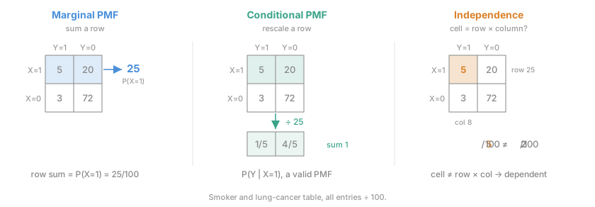
Marginal PMF: sum a row

$P(X=x) = \sum_y P(X=x, Y=y).$

The event $\{X=x\}$ is the union of the disjoint cells "$X=x$ with $Y$ anything", so summing them is just the rule for a disjoint union. This move runs one way only. Joint to marginals is easy summing, marginals back to joint is impossible without relationship information. That is the opening question again.

Conditional PMF: rescale a row

Sample a random adult male: $X=1$ if he currently smokes, $Y=1$ if he develops lung cancer.

Learning $X=1$ keeps only the top row, whose total mass is 25/100. Divide each cell by that total and the row becomes a valid PMF:

A Venn diagram is the wrong tool for this. A circle in a Venn diagram stands for one whole event, but the conditional PMF needs the event $\{X=1\}$ split across every value of $Y$, cell by cell. Those pieces have no home in a two-circle picture. The table shows exactly them.

The comparison that matters is conditional against marginal. Before learning anything, $P(Y=1) = 8/100$. After learning $X=1$, it jumps to $1/5$. Learning $X$ moved $Y$'s distribution, so the pair is dependent. (The event-level version is in conditional-probability.)

Independence: every cell factors

Three equivalent faces:

1. CDF face: the joint cumulative distribution function factors, $F(x,y) = F_X(x)\,F_Y(y)$ for all $x, y$.
2. PMF face: every cell equals its row margin times its column margin, $P(X=x, Y=y) = P(X=x)\,P(Y=y)$. This is the one case where the marginals do fix the joint.
3. Conditional face: $P(Y=y \mid X=x) = P(Y=y)$ whenever $P(X=x) > 0$. Every row renormalizes to the same marginal, so conditioning changes nothing.

The two directions cost differently: one non-factoring cell is enough to disprove independence, but proving it requires every one of the $|X| \cdot |Y|$ cells to factor.

Bayes' rule and the Law of Total Probability (LOTP) hold on PMFs unchanged, with events replaced by "variable $=$ value":

$P(Y=y \mid X=x) = \frac{P(X=x \mid Y=y)\,P(Y=y)}{P(X=x)}, \qquad P(X=x) = \sum_y P(X=x \mid Y=y)\,P(Y=y).$

Chicken and egg: a split Poisson is two independent Poissons

A chicken lays $N \sim \text{Pois}(\lambda)$ eggs. Each egg hatches on its own with probability $p$ and fails with $q = 1-p$. Let $X$ count the hatched eggs and $Y$ the failed ones, so $X + Y = N$. The natural guess is that $X$ and $Y$ are dependent, since $Y = N - X$: learn $X$ and you seem to know something about $Y$. The joint PMF says otherwise.

Given $N = n$, the $n$ eggs are independent trials, so $X \mid N{=}n \sim \text{Bin}(n, p)$. To reach the joint, condition on $N$ with LOTP:

$P(X=i, Y=j) = \sum_{n=0}^{\infty} P(N=n)\,P(X=i, Y=j \mid N=n).$

Given $N = n$, the pair $(i, j)$ is impossible unless $n = i+j$, and once $N = i+j$ and $X = i$, the event $Y = j$ is automatic. So one term survives, and the factorials cancel:

Split every factor along the $i/j$ seam, using $\lambda^{i+j} = \lambda^i \lambda^j$ and $e^{-\lambda} = e^{-\lambda p}\,e^{-\lambda q}$:

$P(X=i, Y=j) = \frac{e^{-\lambda p}(\lambda p)^i}{i!} \cdot \frac{e^{-\lambda q}(\lambda q)^j}{j!}.$

The joint factors into $\text{Pois}(\lambda p) \times \text{Pois}(\lambda q)$. By the PMF face, $X$ and $Y$ are independent.

Two points make this result land. First, $P(X=i)$ is well defined on its own even though only $X \mid N$ was ever specified. Marginalize $Y$ out of the factored joint, the $j$-part sums to 1, and $P(X=i) = e^{-\lambda p}(\lambda p)^i/i!$ with no $N$ in sight. "Not computed yet" is not the same as "not defined": a marginal is one quantity's distribution with the other randomness averaged out, not ignored. This is Poisson thinning: keep each item of a $\text{Pois}(\lambda)$ count independently with probability $p$, and the kept count is $\text{Pois}(\lambda p)$.

Second, the dependence intuition is about the wrong pair. Conditional on $N = n$, the two counts are $\text{Bin}(n,p)$ and $\text{Bin}(n,q)$ and perfectly dependent, knowing one pins the other. Unconditionally, $N$'s Poisson randomness is exactly the kind that makes learning $X$ useless for predicting $Y$. This is special to the Poisson, no other egg-count distribution does it, and it runs both ways: independent $\text{Pois}(\lambda p)$ and $\text{Pois}(\lambda q)$ sum to a $\text{Pois}(\lambda)$ with a binomial conditional, and a Poisson count split by independent coin flips gives back independent Poissons.

The one-time pad: perfect secrecy is independence

Take a message bit $M$ with any adversary prior $P(M=1) = m$, a key bit $K \sim \text{Bern}(1/2)$ independent of $M$, and ciphertext $C = M \oplus K$. The chain rule fills the cells:

where dropping the conditioning is exactly where $K \perp M$ gets used. Without it the table falls apart.

The column sums give $P(C=0) = P(C=1) = 1/2$ whatever $m$ is, and every cell factors as $P(M=i)\,P(C=j)$. So $C \perp M$, the adversary's posterior $P(M=i \mid C=j)$ equals the prior, and seeing the ciphertext teaches them nothing. That is Shannon's perfect secrecy, and it is plain independence, no extra cryptographic machinery.

At real sizes nobody checks $2^n \times 2^n$ cells, the argument goes structural. Fix any pair $(m, c)$: exactly one key $k = m \oplus c$ produces it, and keys are uniform over $2^n$ values, so every row of the giant table is uniform. The table gives the statement to prove, a bijection proves it.

The requirement is identical rows, not a uniform $C$. If every row is the same PMF $D$, LOTP averages identical things and returns that thing:

so conditional equals marginal and posterior equals prior. Uniformity is just what XOR with a uniform key happens to produce. A non-uniform case: append an independent $\text{Bern}(0.9)$ junk bit to every ciphertext. The rows stay identical to each other, the marginal of $C$ is now biased, and the adversary still learns nothing about $M$.

What is still shaky

The seam between conditional and joint quantities. A conditional is not automatically smaller than the marginal, and it is not the joint cell either, the two differ by the row-total factor. The continuous version of this material is built on exactly that move: conditional probability density functions (PDFs) as renormalized slices of a density surface, with integrals in place of row sums. Watch that seam.