joint-distribution-mental-model
The opening question
and are each , and that is everything you know about them. What is ?
Where I got stuck
I answered 1/4 without pausing:
The marked step swaps for , which needs independence, and independence was never given. My justification when pressed: two separate Bernoulli events are independent, right? The belief underneath was that once you know each variable's own distribution, common sense fills in the rest.
A counterexample: flip a single fair coin, let for heads and for tails. Each marginal is , exactly like two separate coins, but
Same marginals, completely different joint.
The key move: one combined sample space, one table
What made the whole picture click was seeing which object the notation commits you to. In my words from the session:
The aha, in my words (lightly cleaned) Even if X and Y have different random experiments underneath, when we write P(X=i, Y=j) we're talking about the probability distribution over the "combined sample space" (the cartesian product of the two sample spaces). It's a function of two variables, as opposed to the usual one-variable function for standard r.v.s. And on this combined sample space we always need to define all r.v.s for each event. That is, we need to write X=i, Y=j. Not just X=i!!! We're moving between underlying experiments when we talk about P(X=i) vs P(X=i, Y=j).
One refinement: there is no moving between spaces. The moment you write , both variables are mappings on one common sample space, and "two different experiments" just means is the product of the two experiments' outcomes. lives on that same space too, as the event " and anything".
This is also what makes comparing the two variables legal at all. I raised it twice as a side worry: how can you write or when they come from different experiments? Once both are mappings on the one combined space, is just the ordinary event , so the comparison is fine the moment a joint model exists.
Draw that space as a 2D table: rows for 's values, columns for 's, one cell per pair. Each outcome lands in exactly one cell, so the cells are mutually exclusive and exhaustive. They partition the space and sum to 1. Getting a marginal is then just projecting the table onto one axis: sum a row and you have collapsed away, which is exactly what means.
Three worlds, same marginals
That projection runs one way only. Keep both marginals pinned at and change only the relationship:
| relationship | |
|---|---|
| (same coin, opposite faces) | |
| independent (two separate coins) | |
| (same coin, same face) |
The chain rule shows this is the full range. is pinned by the marginal, and can be pushed anywhere from 0 to 1, so the joint value sweeps . Finding the top end also corrected a second belief: conditioning does not always shrink a probability, since gives , larger than the marginal .
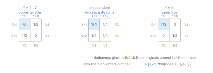
The three tables have identical row and column margins but different interiors. The marginals cannot tell them apart. The joint table is the only object that can. So the honest answer to the opening question is "cannot be determined." Asking two marginals to produce a joint value is asking two shadows to rebuild the object that cast them.
The relationship information lives nowhere inside the two marginal probability mass functions (PMFs), which are just two lists of numbers, one per variable. Even "they come from different experiments" is relationship information you add to the model, never something you read off the marginals. Independence is the one case where the shadows do rebuild the object, and only because "independent" is itself the relationship being handed to you: the joint is then declared to be the product of the marginals (the PMF face in discrete-joint-distributions).
Mantra: marginals are shadows, the joint is the object. Shadows fall out of the object by projection. No pair of shadows gives the object back.