pdf-and-cdf-basics

Tue Jul 14 2026

From staircase to ramp

In the discrete world (probability-distributions-and-random-variables) the CDF is a staircase and the PMF lives in the jumps: $P(X = x) = F(x) - F(x^-)$, the jump height at $x$. A continuous CDF is a smooth ramp with no jumps at all. Apply the same jump formula and it forces $P(X = x) = 0$ for every single $x$. Nothing is left over for any individual point.

The interesting part is what falls out on the way. Writing the small difference at $x$ gives $F'(x)\,dx$, and as $dx \rightarrow 0 \implies P(X = x) = F'(x).dx \rightarrow 0$. It is the chapter's central object: $f(x) = F'(x)$, the probability density function.

One cheap consequence worth pocketing: since endpoints carry zero, $P(a < X < b) = P(a \le X \le b)$, and every half-open version in between. No more $<$ vs $\le$ anxiety.

Probability lives on segments (the dx view)

$f(x)$ is not a probability. $f(x)\,dx$ is: the probability that $X$ lands in a tiny window of width $dx$ around $x$. Density is probability per unit length, which means it carries units. My waiting-time example: $X$ uniform on half an hour has density height 2 measured in hours and height 1/30 measured in minutes. Same random variable, same probabilities, different heights. Only height times width is real.

That also settles why a density can exceed 1. The only validity conditions are $f \ge 0$ everywhere and total area 1. Height 2 (or 3, or 100) is fine as long as the support is narrow enough. $\text{Unif}(0, 1/3)$ sits at height 3 everywhere and is a perfectly legal distribution. The mantra: height is probability per unit length, only area is probability.

The same view is the right way to think about transformations. To understand $Y = g(X)$, don't ask where a point goes, ask what happens to a small segment. The map $g$ sends $[x, x + dx]$ to a segment around $g(x)$, and the probability mass $f(x)\,dx$ riding on it is conserved. If the segment gets stretched, that mass spreads over more length, so the density drops. Compressed, the density rises.

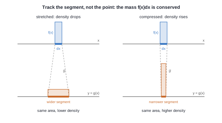
3blue1brown has a video on exactly this segment intuition, from his probability playlist.

Working with densities

The practical workflow: differentiate the CDF when you want the shape, use the CDF directly when you want a probability. The Rayleigh warm-up shows both. Its CDF is $F(x) = 1 - e^{-x^2/2}$ for $x > 0$, so the density is $f(x) = x\,e^{-x^2/2}$ by the chain rule, and the tail needs no integral at all: $P(X > 2) = 1 - F(2) = e^{-2}$. The CDF already did the integrating.

Everything from the discrete world translates with one mechanical dictionary: sums become integrals, $P(X = x)$ becomes $f(x)\,dx$. So $E(X) = \int x\,f(x)\,dx$ and LOTUS reads $E(g(X)) = \int g(x)\,f(x)\,dx$. Linearity, LOTUS, and the variance identity from lotus-and-variance all carry over unchanged.

The Uniform

$\text{Unif}(a, b)$ formalizes "a completely random number between $a$ and $b$": a flat density $f(x) = 1/(b-a)$ on the support, forced by area 1, and a ramp CDF $F(x) = (x-a)/(b-a)$ there. My first CDF attempt failed the standard sanity checks, so they are worth naming: $F$ must be 0 at the left edge, 1 at the right edge, and it must stay at those values outside the support. Writing "0 otherwise" claims $P(U \le 5) = 0$ for $\text{Unif}(0,1)$, which no CDF can do.

For $U \sim \text{Unif}(0,1)$, probability literally is length: $P(U \in (0.2, 0.5)) = 0.3$. Its moments are $E(U) = 1/2$ and $\text{Var}(U) = 1/12$. The general case needs zero new integrals: $a + (b-a)U \sim \text{Unif}(a,b)$ (stretch, then shift), so $E = (a+b)/2$ and $\text{Var} = (b-a)^2/12$. The variance contains only the width $b - a$. Where the interval sits doesn't matter, only how wide the room is.

Same support is not same distribution: the U² trap

A friend argues: $U^2$ still lands in $(0,1)$, so it is still completely random there. The test comes from the Uniform section: completely random means flat PDF, which means linear CDF. Compute it: $P(U^2 \le x) = P(U \le \sqrt{x}) = \sqrt{x}$. Not linear. Same support, different distribution.

The segment view says where the mass went. Squaring pulls every value in $(0,1)$ downward, compressing segments near 0, so the density piles up there. About 70% of draws land below 1/2, since $\sqrt{1/2} \approx 0.707$.

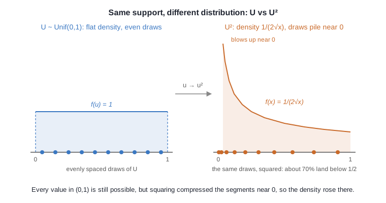
This is exactly the classic nonce-bias bug in ECDSA and Schnorr. Reduce a uniform 256-bit number mod the group order $n$ and every residue is still possible, but residues below $2^{256} \bmod n$ get hit slightly more often. The support looks fine, the distribution is not uniform, and with enough signatures lattice attacks turn that tiny skew into the secret key. The flat-PDF test is the formal version of the check that catches it.

Universality of the Uniform

One theorem, two directions, both riding on the Uniform's special property: its CDF is the identity, $P(U \le p) = p$, so $U$ can hand you an event of any probability you name.

Direction 1: $F^{-1}(U)$ has CDF $F$. I want $X = g(U)$ with $P(X \le x) = F(x)$. Solve for $g$ instead of verifying a given answer:

$P(g(U) \le x) = P(U \le g^{-1}(x)) = g^{-1}(x),$

so matching against $F(x)$ forces $g^{-1} = F$, that is $X = F^{-1}(U)$. The first step silently used that $g$ is increasing, which is why the theorem assumes $F$ strictly increasing.

My own reading of what the proof does: we have a family of events $\{X \le x\}$ whose probabilities we want to be $F(x)$. The Uniform has the special property $P(U \le u) = u$, so in particular $P(U \le F(x)) = F(x)$, an event with exactly the right probability, sitting there pre-made. Setting $X = F^{-1}(U)$ just lines $\{X \le x\}$ up with $\{U \le F(x)\}$. The important property is realizing $P(U \le F(x)) = F(x)$. That is the core of the proof.

The percentile reading makes the result feel obvious: a CDF converts values to percentiles, $F^{-1}$ is the percentile-to-value lookup, and to draw from any distribution you draw a percentile uniformly and look up which value owns it.

The picture is uniform rain on the percentile axis:

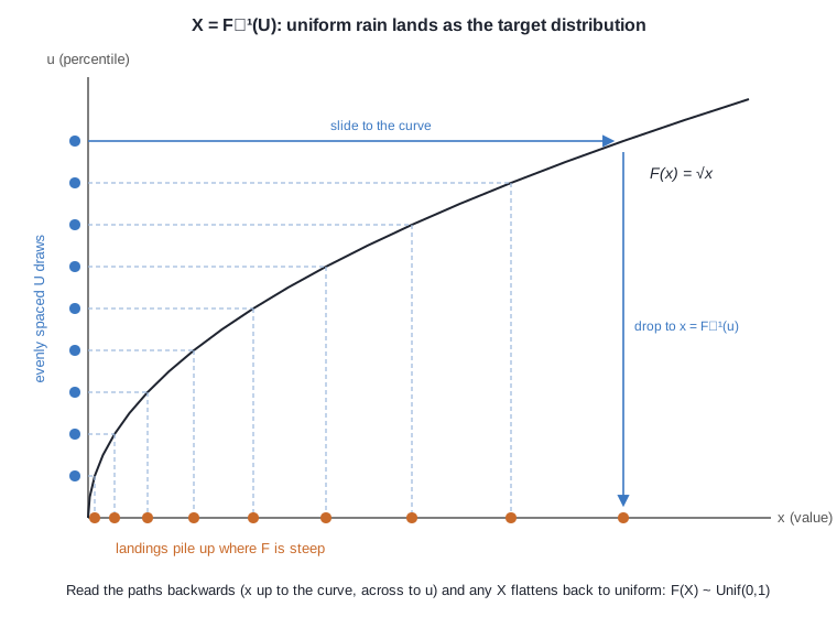
Where $F$ is steep, a wide band of percentiles gets squeezed into a narrow window of values, so landings pile up exactly where the density is tall. The slope $F' = f$ is the local compression ratio of this transport, the segment view from above, one more time. And $U^2$ was already this machine running: target $F(x) = \sqrt{x}$ gives $F^{-1}(u) = u^2$.

Direction 2: $F(X) \sim \text{Unif}(0,1)$. Feed $X$ into its own CDF and it flattens, whatever distribution $X$ had. One line, using that a strictly increasing $F$ makes $\{F(X) \le u\}$ and $\{X \le F^{-1}(u)\}$ the same event:

$P(F(X) \le u) = P(X \le F^{-1}(u)) = F(F^{-1}(u)) = u.$

You never invert $F$ inside a probability, you just rename the event: both descriptions represent the same values underneath, because $F$ is a simple one-one mapping $x \to F(x)$. Strict monotonicity is what makes the renaming valid in both directions.

Why $(0,1)$ and not some $\text{Unif}(a,b)$? In direction 2 it is forced: $F$ outputs probabilities, so $F(X)$ physically lives in $[0,1]$. In direction 1 it is just the canonical choice. From a $V \sim \text{Unif}(a,b)$ source, standardize first and use $X = F^{-1}\big((V-a)/(b-a)\big)$. Direction 1 is what simulation libraries call inverse transform sampling: computers only generate uniform bits, and this is how uniform bits become samples from anything with a tractable $F^{-1}$.

What stayed shaky

The sitting's one real miss: I claimed neither probability nor $dx$ has units. Probability is a pure number, but $dx$ is a length in $X$'s units, and that is what makes density a per-unit-length quantity. The re-test for next week: is the hours-to-minutes rescaling (height 2 vs height 1/30) still obvious? If yes, the density concept is durably in.