normal-and-exponential-distributions
The sitting in one line Both named distributions are one simple object plus a transport rule. The Normal is a single bell, stretched by and slid to , with every question routed back to . The Exponential is the survival function , and memorylessness is why nothing else could do its job.
The standard Normal
The standard Normal has PDF
The exponent is just . The is the normalizing constant, which exists only to make the total area 1. This PDF is special enough to get its own letter , and its CDF gets .
The mean is where the symmetry pays out. The expectation integrand is an odd function: same magnitude at , opposite sign, so the positive lobe cancels the negative lobe and with no antiderivative in sight. One footnote makes the cancellation legal: each lobe must be finite ( is undefined), and it is, because dies faster than any polynomial grows. The same argument kills every odd moment ( for odd , so too). Variance takes an integration by parts I took on faith: , hence the notation .
has no closed form, so all practical work runs through identities. The first one: anchor at , name the slab between and , and the bookkeeping lands on
The mental handle: the left tail below equals the right tail above , so .
Transforms move mass, not points
A transform of a random variable moves probability mass, and the only honest way to follow it is to track a small segment, never a point. This is the view from pdf-and-cdf-basics doing real work.
The warm-up was . My flipping argument: negation literally maps to , so the PDF flips over 0, and is even, so too. The argument is valid, but it rests on a hidden lemma worth saying out loud: negation carries the mass sitting on onto , an interval of the same width. Rigid transport, no stretching, so heights carry over unchanged. (The CDF route needs no picture at all: . Two moves.)
The width caveat is the whole story. Run the same flip on and it breaks: the segment lands on , whose width is to first order. The width multiplier is the derivative of the map. To keep the mass block's area fixed, the height divides by that same factor: . Near 0, where , widths compress and the density piles up instead. That is the pile-up from sitting 1, now with a formula behind it.
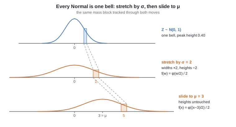
The general Normal is defined by this transport. Take in two stages. Stretch: scales every width by , so heights divide by , giving . Shift: sliding by moves the curve without touching widths, giving
Why and not ? Read it from the new variable's side. The height that lived at now lives at , so the density at is the original looked up at its preimage : from 's perspective, holds whatever lived at . The shift is the same logic, the mass at came from . The recipe for any one-to-one : evaluate the old density at the preimage, then divide by the stretch factor .
Standardization and the 68-95-99.7 rule
The transport also runs backwards: if then , and consequently . There is only one Normal, and every Normal question becomes a question. For quick mental math: , , .
The worked pipeline: , find . First trap dodged: the second parameter is the variance, so , not 4. Standardizing turns into , so the exact answer is by the tail identity. For the approximation, my decomposition: is the left half of the 1SD band (0.34) and is the right half of the 2SD band (0.475), total 0.815 against a true 0.8186. The bands measure from , not from 0. That is exactly what standardizing guards against.
The crypto anchor: Gaussians carry lattice crypto. Falcon samples discrete Gaussians, LWE hides secrets under Gaussian noise, and the security arguments are tail bounds, the 68-95-99.7 rule taken to cryptographic extremes.
The Exponential from its survival function
The Exponential models the waiting time until the first arrival when arrivals hit at rate . My recall worry ("doesn't blow up on the left?") is answered by the story: waits are never negative, the support is , and the blow-up region is simply not in it. The kernel needs a constant, and unlike the Normal's this one is a freshman integral: , so
Units sanity check: carries per-time units, exactly the density units a PDF over time must have, and in the exponent is dimensionless.
The CDF is , so the survival function is . That survival function is the real primitive: exponential-survival-first rebuilds it from nothing but a constant rate, and everything below runs through it.
The mean and variance come from the chapter's signature move, compute for the simplest family member and transform out. One integration by parts gives for , and taking on faith gives . Scaling is the family's only knob (a shift would drag the support off , so unlike the Normal there is no location part): , with mean and variance . Faster arrivals, shorter waits. One flag from my own work: I wrote and got the right number only because is its own square. The formula is . Cheap luck, flagged.
Memorylessness
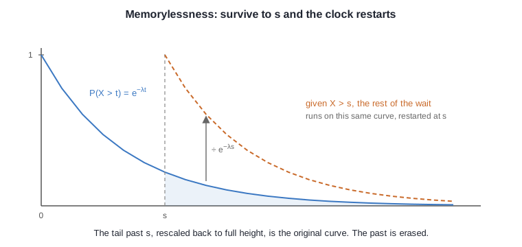
Memoryless property A continuous distribution on is memoryless if for all : Given you have already waited without success, the chance of surviving another is a fresh start. The past is erased.
The proof is two lines once you see the collapse: the event implies , so their intersection is just the smaller event, and the conditional becomes a ratio of survivals:
What the whole proof rests on, in one sentence: exponential functions have the property . The survival function factorizes, so conditioning divides the past out exactly. No polynomial or Gaussian tail survives that ratio unchanged. And the converse holds: any continuous distribution on whose survival function satisfies is forced to be for some . So the Exponential is the only memoryless continuous distribution. Memorylessness characterizes it.
The Poisson bridge
Poisson process with rate λ Arrivals land on a timeline such that the number of arrivals in any interval of length is , and counts in disjoint intervals are independent.
The definition speaks only the counting language (how many arrivals, a discrete number). The waiting language is one sentence away: "the first arrival has not happened by time " is the same event as "zero arrivals landed in ". Identical events have identical probabilities, so
The Exponential survival function falls out of a definition that never mentioned waiting: . After the first arrival, independence of disjoint intervals restarts the process fresh, so the gaps between arrivals are i.i.d. . (Disjoint is doing the work there: overlapping intervals share arrivals, so their counts are obviously dependent.) One process, two views: count the arrivals and you get Poisson, time them and you get Exponential. That is why they share the letter .
The units wire I crossed twice before it settled: is a rate (arrivals per unit time), is a time. Reciprocals, not equals. Buses at rate 6 per hour have mean gap hour, and . They coincide only at , the deceptive special case. The other , the prefactor in , is the same letter doing a second consistent job: the density's per-time units showing up for work.
Bitcoin runs on this bridge. Block arrivals are engineered into a Poisson process (difficulty retargets to hold per minute), inter-block gaps are , and memorylessness is what "progress-free mining" means. After 25 minutes without a block, the expected wait is still 10 minutes from now. A block is never "due".
What stayed shaky: Fred's bus paradox
Buses in Blotchville have Expo gaps with mean 10 minutes, Fred arrives at a random moment, and memorylessness resets the clock: his expected wait is a fresh 10 minutes. His friend argues 5, and each premise sounds fine (you land uniformly inside a gap, the average gap is 10, so you wait half of it). The part I did get: with alternating 50/5 gaps, the dart lands in a 50-minute gap ten times more often, so the gap containing Fred is systematically longer than a typical gap. Length-biased sampling. Which sentence of the friend's argument actually dies, and how the two answers reconcile, is parked as fred-bus-waiting-paradox and opens sitting 3.